

View on GitHub
Open this notebook in GitHub to run it yourself
Quantum computational finance: quantum algorithm for portfolio optimization
In this tutorial, we will work through a concrete example of portfolio optimization. Our goal is to determine how to allocate capital across several assets so that we control risk while still aiming for good returns. To do this, we use historical stock price data to construct a portfolio, that is, the allocation ratios of the assets. The approach is motivated by the methods proposed in References [1,2], where portfolio optimization is identified as a problem that can potentially be accelerated using the HHL algorithm. As a simple practical example, we consider an investment in four major technology stocks and examine how to distribute capital among them in an effective way. first we need to install some out package to collect stock data.Loading Dataset of Stock
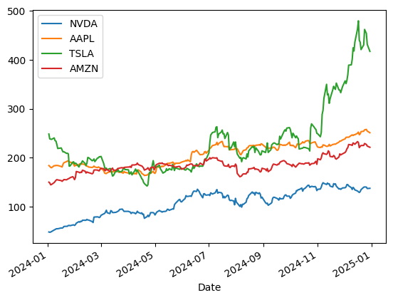
We define csv_data which was generated fromyfinance. We use the data from 2024-01-02 to 2024-12-30.
Output:
Plot the stock price of selected stock
Output:
Conversion to Daily Returns
The daily return (rate of change) of an individual stock is defined as follows, letting be the date: It is obtained usingpct_change() in pandas.
| AAPL | AMZN | NVDA | TSLA | |
|---|---|---|---|---|
| Date | ||||
| --- | --- | --- | --- | --- |
| 2024-12-23 | 0.003079 | 0.000622 | 0.036908 | 0.022681 |
| 2024-12-24 | 0.011451 | 0.017774 | 0.003939 | 0.073549 |
| 2024-12-26 | 0.003190 | -0.008732 | -0.002069 | -0.017609 |
| 2024-12-27 | -0.013264 | -0.014534 | -0.020874 | -0.049479 |
| 2024-12-30 | -0.013245 | -0.010950 | 0.003504 | -0.033012 |
Expected Return
Calculate the expected return for each stock. Here, the arithmetic mean of historical returns is used.Output:
Variance-Covariance Matrix
The sample unbiased variance-covariance matrix of returns, , is defined as follows:- Let the return of each asset be the random variable .
- The covariance is:
- The matrix aggregating this for all assets is :
| AAPL | AMZN | NVDA | TSLA | |
|---|---|---|---|---|
| AAPL | 0.050204 | 0.021167 | 0.029819 | 0.046741 |
| AMZN | 0.021167 | 0.078892 | 0.064226 | 0.056531 |
| NVDA | 0.029819 | 0.064226 | 0.274981 | 0.071096 |
| TSLA | 0.046741 | 0.056531 | 0.071096 | 0.403576 |
Portfolio Optimization
Having defined the necessary variables, we now proceed to actual portfolio optimization. We represent the portfolio as a -component vector . This represents the proportion of holdings in each stock; for example, implies a portfolio where of total assets are invested in AAPL stock. Consider a portfolio that satisfies the following equation:- The diagonal elements are the variances of each asset (intensity of risk).
- The off-diagonal elements are the covariances between assets (strength of correlation).
- The expected return of the portfolio (average value of returns) is .
- The sum of the weights invested in the portfolio is 1 ().
Lagrange Multiplier Method in Mathematical Optimization
The mathematical optimization problem described above is an optimization problem with equality constraints. By solving this using the Method of Lagrange Multipliers, we can find candidates for the local optimal solution. The Method of Lagrange Multipliers is defined as follows: Here, represents the objective function, and the second term represents the constraint functions. are the Lagrange multipliers. In the case of our portfolio optimization problem, if we introduce Lagrange multipliers and , the Lagrangian is given by: Since the constraints are linear equations, the optimal solution is guaranteed by just the first-order derivatives. Therefore, we differentiate the Lagrangian function above with respect to the variables .First-Order Optimality Conditions (KKT Conditions)
Organizing as a System of Linear Equations
If we organize (A) through (C) into a linear equation regarding the unknowns , we get: Looking at this row by row:- 1st Row: (Expected Return Constraint)
- 2nd Row: (Sum of Weights = 1 Constraint)
- 3rd Row: (Stationarity Condition)
Preprocessing for HHL
Construction of matrix
Output:
Construction of Vector
Output:
Redefining the Matrix
Typically, the matrix formulation for HHL assumes a standard form with the following properties:- The right-hand side vector is normalized.
- The matrix has a size of .
- The matrix is Hermitian.
- The eigenvalues of matrix lie within the range .
1) Normalized b
As preprocessing, normalize and then return the normalization factor as postprocessing.2) Make the Matrix of Size
Complete the matrix dimension to the closest with an identity matrix. The vector is completed with zeros. However, our matrix is already the right size.Output:
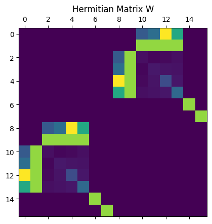
3) Hermitian Matrix
Symmetrize the problem: This increases the number of qubits by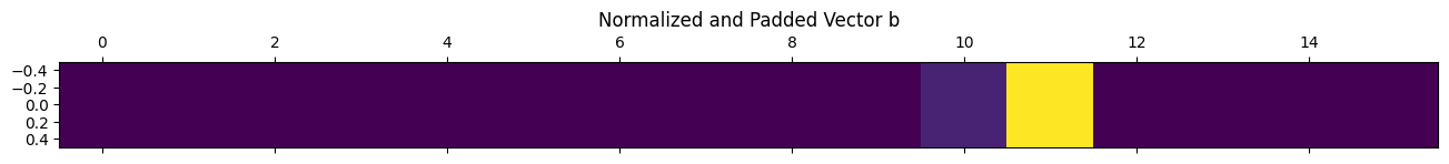
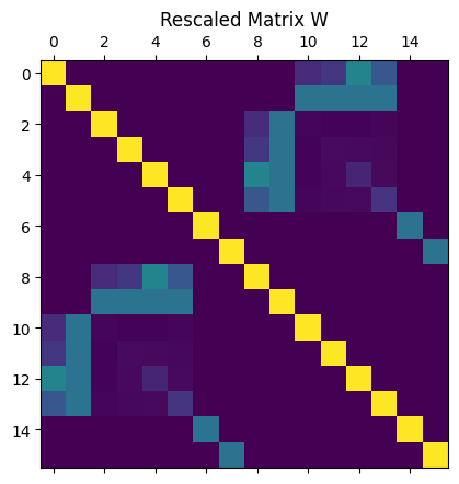
4) Rescaled Matrix
If the eigenvalues of matrix lie within the interval , we can handle this by transforming the matrix and then reverting the result. The transformation is defined as follows: In this case, the eigenvalues of fall within the interval . The relationship with the eigenvalues of the original matrix is given by: Where is the eigenvalue of obtained by the QPE (Quantum Phase Estimation) algorithm. This correspondence between eigenvalues is used in the formula for eigenvalue inversion within theAmplitudeLoading function.
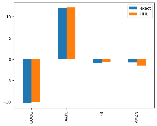
Defining HHL Algorithm for the Quantum Solution
This section is based on Classiq HHL in the user guide, here and here. Note the rescaling insimple_eig_inv based on the matrix rescaling.
Output:
Output:
Output:
Output:
Output:
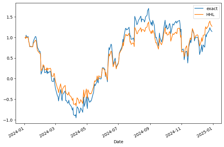
| exact | HHL | |
|---|---|---|
| Date | ||
| --- | --- | --- |
| 2024-01-02 | -325.764298 | -421.744540 |
| 2024-01-03 | -320.943657 | -410.339168 |
| 2024-01-04 | -344.106605 | -433.974406 |
| 2024-01-05 | -329.292530 | -418.664555 |
| 2024-01-08 | -332.896116 | -421.666555 |
Output:
Output:
Reference
- [1] P. Rebentrost and S. Lloyd, “Quantum computational finance: quantum algorithm for portfolio optimization“, https://arxiv.org/abs/1811.03975
- [2] 7-3. Portfolio optimization using HHL algorithm: https://dojo.qulacs.org/en/latest/notebooks/7.3_application_of_HHL_algorithm.html